
Last updated on 14/01/2024
The world is being hit hard by the Covid-19 (or SARS-CoV-2 or just Coronavirus, as most people call it) pandemic. The number of cases and deaths is skyrocketing worldwide.
Epidemiologists and data scientists resort to multi-factorial models to predict the dynamics of the outbreak. Simpler tools can be used to look for trends just fitting epidemiological data.
The simplest models are based on either polynomial (second or higher order) or exponential functions. Both of them can provide a reasonable fitting during the first days of the outbreak, but not for long, as both of them diverge to infinity with time, while the total cases or deaths and infections should plateau to a value that cannot exceed the number of people in a given country.
A more accurate model is based on the Logistic function, which belongs to the wider class of the so-called sigmoid functions, all sporting a typical S-shaped behaviour, asymptotically saturating to a max value.
With the Matlab script described hereafter, you will be able to generate fitting plots as the ones shown below, using your own data.
Let’s see how infection data can be fitted in Matlab using the Logistic function.


The analytical expression of our function is:

First of all, we need some data to fit.
In this Excel file you find example data, describing the Covid-19 outbreak in Italy in the past days. The structure of the file should be quite self-explaining.
If you want to use your own data, there are several reliable sources of information, such as the World Health Organization website, or this one, very convenient.
The Matlab script described in the following will show you how such data can be fitted using the Logistic function and its derivative.
% Matlab script to fit the number of total cases and infections using
% the logistic function: A/(1+exp(-B*(x-C))).
%
% Once the coefficients A, B e C are found, the (time) derivative is computed and the rate of
% change is compared with actual data about new cases and new deaths.
%
% Singapore, March 13 and 14, 2020
clear all
clc
close all
% "day" is the variable counting days in the observation interval.
% The range of "day" is from 1 to "Last_day"
Last_day = 60; % This number can be free
prev_day = 1:Last_day;
Data_from_spreadsheet = readtable("covid_data.xlsx");
% Let's check the size of the table read from Excel.
% "num_day" is the number of days considered.
[num_day,D2] = size(Data_from_spreadsheet);
% Let's convert the data in the table into a matrix "Data":
Data = Data_from_spreadsheet{1:num_day,2:5};
day = [1:num_day]';
today = max(day);
cases = Data(:,1);
new_cases = Data(:,2);
deaths = Data(:,3);
new_deaths = Data(:,4);
% =============================================================
% Let's find the coefficients of the logistic function by fitting data
% about total cases:
ft = fittype( 'a/(1+exp(-b*(x-c)))', 'independent', 'x', 'dependent', 'y' );
opts = fitoptions( 'Method', 'NonlinearLeastSquares' );
opts.Display = 'Off';
% We need to provide some guess values to the algorithm to find
% the 3 coefficients (a, b, c).
% The fitting algorithm does not always converge. Choosing proper guess values
% is important.
opts.StartPoint = [70000 0.25 30];
% Data fitting:
[fitresult, gof] = fit( day, cases, ft, opts );
A = fitresult.a;
B = fitresult.b;
C = fitresult.c;
% Total cases according to fitting (logistic function):
prev = A./(1+exp(-B.*(prev_day-C)));
% New cases per day (derivative of logistic function, analytically computed):
derivative = A.*B.*exp(-B.*(prev_day-C))./(exp(-B.*(prev_day-C))+1).^2;
hold on
plot(prev_day,prev); %figure 1
plot(day,cases,'ro');
% Let's plot a horizontal line corresponding to the asymptot :
yline(A,'-.r');
% Let's report the R^2 on the plot:
text(today/3,max(prev)/2,strcat("R^2 = ",num2str(gof.rsquare)));
text(today/3,A*1.05,strcat("Total cases = ",num2str(round(A))));
%ylim([0 1.1*A]); %could be useful to set the range of values on the y-axis
title("Total cases (fitting with Logistic function)");
xlabel("Day");
hold off
figure
hold on
plot(prev_day,derivative,'b'); grid on %this creates figure 2
plot(day,new_cases,'ro');
hold off
xline(today,'-.r');
[Max,Index] = max(derivative); %this spots the max value
xline(Index);
text(Index,Max,strcat(" Peak: ",num2str(round(Max))," cases/day (day ",num2str(Index),")"));
%ylim([0 1.1*Max]);
title("New cases per day (derivative of Logistic function)");
xlabel("Day");
text(today,Max*0.1,strcat("Today: day ",num2str(today)));
% ======== let's repeat the same but for deaths ==========
ftM = fittype( 'a/(1+exp(-b*(x-c)))', 'independent', 'x', 'dependent', 'y' );
optsM = fitoptions( 'Method', 'NonlinearLeastSquares' );
optsM.Display = 'Off';
optsM.StartPoint = [10000 0.25 30];
% Data fitting:
[fitresultM, gofM] = fit( day, deaths, ftM, optsM );
AM = fitresultM.a;
BM = fitresultM.b;
CM = fitresultM.c;
% Total deaths according to fitting
prevM = AM./(1+exp(-BM.*(prev_day-CM)));
derivativeM = AM.*BM.*exp(-BM.*(prev_day-CM))./(exp(-BM.*(prev_day-CM))+1).^2;
figure
hold on
plot(prev_day,prevM); % this creates fig 3
plot(day,deaths,'ro');
% Horizontal asymptote:
yline(AM,'-.r');
text(today/3,max(prevM)/2,strcat("R^2 = ",num2str(gofM.rsquare)));
text(today/3,AM*1.05,strcat("Total deaths = ",num2str(round(AM))));
%ylim([0 1.1*AM]);
title("Total deaths (fitting with Logistic function)");
xlabel("Day")
hold off
figure
hold on
plot(prev_day,derivativeM,'b'); grid on % this creates fig 4
plot(day,new_deaths,'ro');
hold off
xline(today,'-.r');
[MaxM,IndexM] = max(derivativeM);
xline(IndexM);
text(IndexM,MaxM,strcat(" Peak: ",num2str(round(MaxM))," deaths/day (day ",num2str(IndexM),")"));
%ylim([0 1.1*MaxM]);
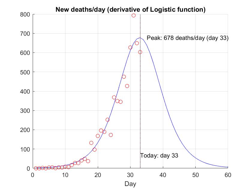
title("New deaths/day (derivative of Logistic function)");
xlabel("Day");
text(today,MaxM*0.1,strcat("Today: day ",num2str(today)));


